The simplest neural network using pytorch

Building a neural network from scratch might seem intimidating, but it is quite simple using pytorch. In this post, I will slowly build up to creating a very simple neural network that approximates the quadratic relationship between two variables, starting from the very basics. I will talk about

• Using gradient descent to approximate polynomial functions using pytorch tensors.
• Doing the same using the pytorch.nn module.

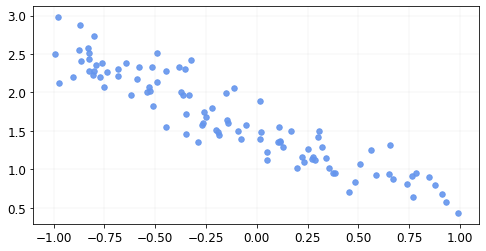
We will start with a very simple linear relationship between variables. Let’s say we have an independent variable \(x\) and a dependent variable \(y\) (both scalars) that depends upon \(x\) according to the equation \( y = ax+b+ \epsilon. \) where \(\epsilon\) is the error term. We only have observations for \(x\) and \(y\) and we are interested in estimating \(a\) and \(b\) such that we minimize the mean squared error between the original \(y\)s and the predicted \(\hat{y}\) using the estimated \(\hat{a}\) and \(\hat{b}\). I know what you are thinking - we can use ordinary least squares regression from statsmodels or R. Yes, we can but we will do it ourselves. We will do it using gradient descent

Let’s first generate some data.

n = 100
x = torch.ones(n,2) 
x[:,0].uniform_(-1.,1) #replace ones by uniformly generated numbers between -1 and 1 inplace. 
x[:5]

tensor([[ 0.9764,  1.0000],
        [ 0.8581,  1.0000],
        [-0.4236,  1.0000],
        [-0.7678,  1.0000],
        [ 0.2261,  1.0000]])

The first column above represents the x values, and the second is just a constant that will be multiplied by \(b\).

Let’s now define a tensor to contain \(a\) and \(b\).

coef = torch.tensor([-1.,1.5]); 
errors = torch.empty(n).normal_(mean=0,std=0.25)
y = x@coef + errors
y[:5]

tensor([0.5731, 0.7709, 1.6031, 2.4825, 1.3974])

The data looks like this

Let’s define a function that calculates the mean squared error between the original and the predicted \(y\)s.

def mse(y, y_hat): return ((y - y_hat)**2).mean()

To estimate \(a\) and \(b\), we will start with a random guess, calculate the value of the MSE at those values of \(a\) and \(b\), calculate the gradient of MSE with respect to each variable at that value, and then subtract a small proportion of that gradient from the corresponding estimate, and iterate. That’s gradient descent.

pytorch really makes this process easy by calculating the gradients for us. All we need to do is to tell pytorch which quantity we need the gradients for and with respect to what variables.

Let’s start with a random estimate.

coef_hat = torch.tensor([2.,1], requires_grad= True) #estimates of a and b || tell pytorch we need the gradients. 

Let’s see what our estimated \(y\)s look like with these values of \(a\) and \(b\).

y_hat = x@coef_hat

The mean squared error is

loss = mse(y, y_hat); loss.data

tensor(3.5852)

Now we need the gradients of the loss (MSE) with respect to our variables stored in coef_hat.

loss.backward()

By running this command, pytorch automatically calculated the gradients for the variables that we asked for (by setting requires_grad=True) that were used for the computation of loss. We can look at the values

coef_hat.grad

tensor([ 2.2119, -0.8841])

To subtract a proportion of the gradients from the current estimates, we do

with torch.no_grad():
    coef_hat -= (0.5 * coef_hat.grad) # subtract 50% of the gradient from current estimate
    coef_hat.grad.zero_()

After we subtract, we tell pytorch that we have used the gradients and you can set them to zero for the next computation. If we don’t do it, the gradients from the next iteration will be added to these instead of replacing these. The proportion of gradients that we subtract from the estimates at each iteration is known as the lr (learning rate), which in this case we set to 50% or 0.5. Note that for most practical applications, 0.5 is too big, but we will use 0.5 for the purpose of this illustration.

After one iteration, our predictions are closer to the data than what we started with in terms of the mean squared error. The loss now is

mse(y, x@coef_hat.data)

tensor(1.3834)

We will repeat this process a number of times and see how our predictions look.

lr = 0.5
for i in range(20):
    y_hat = x@coef_hat
    loss = mse(y, y_hat)
    loss.backward()
    with torch.no_grad():
        coef_hat.sub_(lr * coef_hat.grad)
        coef_hat.grad.zero_()
    if i%5==0: 
        print(f"iter {i}, Loss = {loss.data}");

iter 0, Loss = 1.3834195137023926
iter 5, Loss = 0.06873328238725662
iter 10, Loss = 0.056006383150815964
iter 15, Loss = 0.05588318035006523

The MSE reduced from 1.38 to 0.05. The predictions for these 20 iterations look something like this.

We can look at the estimated values of a and b.

coef_hat

tensor([-0.9967,  1.4863], requires_grad=True)

Let’s now try to do the same thing with a quadratic function of the type \( y = ax^2 + bx + c + \epsilon \)

Like before, we first generate some data.

n = 100
x = torch.ones(n,3) 
x[:,1].uniform_(-1.,1) #replace ones by uniformly generated numbers between -1 and 1 inplace. 
x[:,0] = x[:,1]**2
x[:5]

tensor([[ 0.2638,  0.5137,  1.0000],
        [ 0.6623, -0.8138,  1.0000],
        [ 0.4305, -0.6561,  1.0000],
        [ 0.4266, -0.6532,  1.0000],
        [ 0.0801, -0.2830,  1.0000]])

The middle column above represents the x values, the first one stores the values of \(x^2\).

Let’s now define a tensor that contains \(a,b,\) and \(c\).

coef = torch.tensor([4.,3,2]); 
errors = torch.empty(n).normal_(mean=0,std=0.25)
y = x@coef + errors
y[:5]

tensor([4.6253, 2.1019, 1.5409, 1.4461, 1.7782])

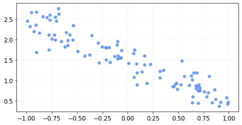
The data looks like this

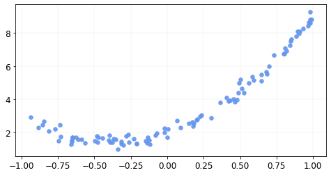
Let’s start with a random estimate

coef_hat = torch.tensor([-5.,-2, 4], requires_grad= True) 
y_hat = x@coef_hat

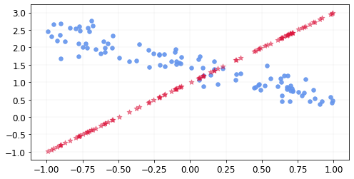
The predictions with our estimates look like this

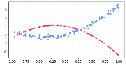
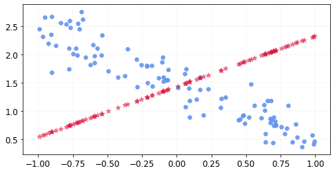
As before, we do gradient descent and our estimates improve over time like shown below.

We can do the same thing for a polynomial of degree 3.

Using gradient descent, we were able to find very good estimates of our coefficients. But note that while estimating our coefficients above, we assumed in each case that we know the shape of the function. For example, for the quadratic relationship, we searched for the best function among a class of all quadratic functions.

In practical applications, we almost never know the shape of the functional relationship between the dependent and the independent variables. This is where neural networks come into play. According to the Universal approximation theorem, simple neural networks can approximate a wide variety of functions given appropriate parameters.

Below, we will see how to build simple neural networks using pytorch.nn that try to approximate the linear and the quadratic relationships.

For the linear case, believe it or not, we have already built a neural network. What we did before for the linear case is a neural network with 0 hidden layers where each input and the corresponding output are 1d tensors of size 1. For such a neural network, we only have 2 parameters that we need to optimize which we already did using gradient descent. Using the pytorch.nn module, the same thing can be done in the following way.

Let’s generate data for x and y like in the linear case above.

x[:5],y[:5]

(tensor([[-0.5180,  1.0000],
         [-0.5119,  1.0000],
         [-0.2702,  1.0000],
         [-0.3556,  1.0000],
         [ 0.2720,  1.0000]]),
 tensor([2.3287, 1.8186, 1.5739, 2.3054, 1.1293]))

#Make them 2d tensors 
x_trn = x[:,0][:,None] 
y_trn = y[:,None]

The data looks like this.

We create a subclass of the nn.Module class as such.

class Linear_Reg(nn.Module):
    def __init__(self):
        super().__init__()
        self.weights = nn.Parameter(torch.randn(1, 1)) #random estimate of a (from y = ax + b)
        self.bias = nn.Parameter(torch.zeros(1))       #random estimate of b 

    def forward(self, xb):
        return xb @ self.weights + self.bias   #define how to process an input xb.

model = Linear_Reg()

model is now a neural network that when given an input will return an output according to it’s forward method. We now need to learn the parameters using gradient descent like before. pytorch’s optim can help us do this. We define the optimizer for our model’s parameters like this

opt = optim.SGD(model.parameters(), lr = 0.5) #lr = learning rate

for i in range(20):
    y_hat = model(x_trn)
    loss = mse(y_trn, y_hat)
    loss.backward()
    opt.step()
    opt.zero_grad()
    if i%5==0: 
        print(f"iter {i}, Loss = {loss.data}");

iter 0, Loss = 6.714003086090088
iter 5, Loss = 0.1343260407447815
iter 10, Loss = 0.05274592712521553
iter 15, Loss = 0.04973254352807999

The predictions improve like this.

This looks exactly the same as before as it should.

Finally, let’s try to approximate the quadratic relationship using a neural network. We can do it the same way as before i.e., make each input \(x\) a 1d tensor of size 2 containing the values \(x\) and \(x^2\), but we want to not do that since we are assuming that we do not know the functional form of the relationship. We will add the non-linearity using the Relu function.

First let’s generate some data using the same method as in the quadratic section above.

x[:5],y[:5]

(tensor([[ 0.8310,  0.9116,  1.0000],
         [ 0.2035, -0.4511,  1.0000],
         [ 0.7908, -0.8892,  1.0000],
         [ 0.4757,  0.6897,  1.0000],
         [ 0.3798,  0.6163,  1.0000]]),
 tensor([4.7228, 2.7561, 4.4042, 3.0588, 3.3131]))

#Make them 2d tensors 
x_trn = x[:,1][:,None] 
y_trn = y[:,None]

The data looks like this

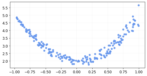
Let’s generate a neural network class like before, but this time, we will add some nonlinearities using Relu. Let’s add one hidden layer with 10 neurons.

class NN_quadratic(nn.Module):
    def __init__(self):
        super().__init__()
        #initialize all parameters that we will need
        self.weights1 = nn.Parameter(torch.randn(1,10))
        self.bias1 = nn.Parameter(torch.zeros(10))
        self.weights2 = nn.Parameter(torch.randn(10,1))
        self.bias2 = nn.Parameter(torch.zeros(1))
        
    def forward(self, xb):
        at_layer1 = F.relu(xb@self.weights1 + self.bias1) # this happens at the hidden layer. 
        return at_layer1@self.weights2 + self.bias2

We create an instance of the above class, and set up the optimizer for it’s parameters

model = NN_quadratic()
opt = optim.SGD(model.parameters(), lr = 5e-2) #lr = learning rate

and train the network. Note that we used a learning rate of 0.05 for this.

for i in range(300):
    y_hat = model(x_trn)
    loss = mse(y_trn, y_hat)
    loss.backward()
    opt.step()
    opt.zero_grad()
    if i%50==0: 
        print(f"iter {i}, Loss = {loss.data}");

iter 0, Loss = 10.352397918701172
iter 50, Loss = 0.0872739851474762
iter 100, Loss = 0.07360737770795822
iter 150, Loss = 0.07017877697944641
iter 200, Loss = 0.06543848663568497
iter 250, Loss = 0.060145407915115356

The predictions improve like this.

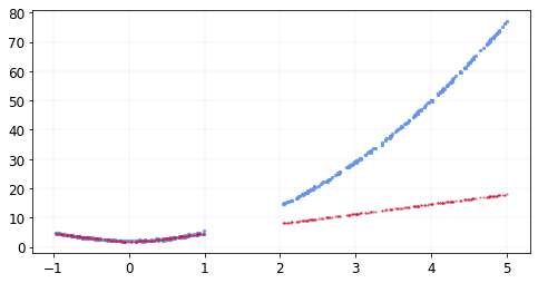
We have built a neural network that approximates the quadratic relationship between two variables. Note that the code can be made even simpler using nn.Linear or nn.Sequential (see this blog for a more comprehensive tutorial on pytorch.nn), but the point of this post was to really understand the basics. Also, please note that we did not talk about overfitting here, which is a very important concept in machine learning. In fact, we can see that the neural network we just trained does not generalize very well to values of x that are greater than 1, but let’s leave that discussion for another post. I hope this post helps you get started with neural networks and pytorch.