Boosting and XGBoost
Boosting is an ensemble algorithm in supervised machine learning that builds a strong learner from multiple weak learners. Unlike bagging, where multiple random samples of the data are drawn and models are trained on those random samples independently, in boosting, models are trained sequentially. The model that is trained in each iteration of boosting tries to correct the errors made by the models in previous iterations. Gradient boosting allows for optimization of arbitrary differentiable loss functions, while still building the strong model in a sequential way like other boosting methods.
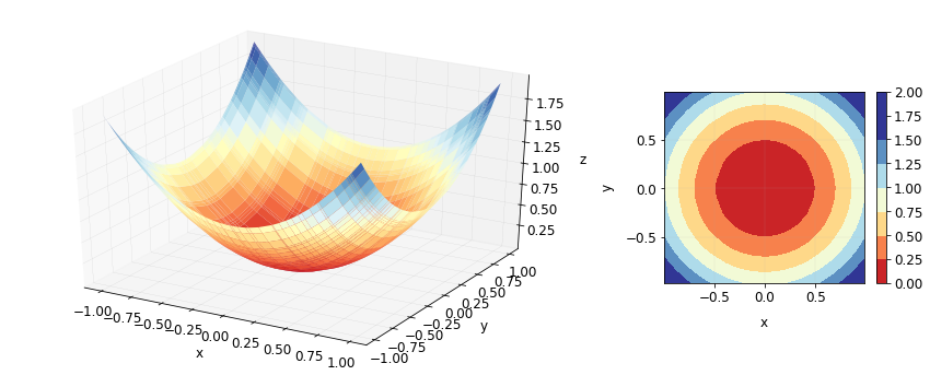
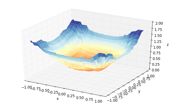
In this post, I will talk about gradient boosting for regression using one of the most popular libraries for gradient boosting, XGBoost. I will try to approximate a simple function \[ f(x,y) = x^2 + y^2\] using gradient boosting. This is the type of exploration I did when I first started playing with gradient boosting. I think doing such simple experiments really helps in becoming familiar with an algorithm and the corresponding library.
Data
Let’s first generate some data.
n = 50
x = np.sort(np.random.uniform(-1., 1, n))
y = np.sort(np.random.uniform(-1., 1, n))
x[:3], y[:3]
(array([-0.99764506, -0.99354683, -0.97877897]),
 array([-0.97193725, -0.924306  , -0.84584719]))
X, Y = np.meshgrid(x, y)
Z = X**2 + Y**2
trn = np.array([X.reshape(-1), Y.reshape(-1)]).transpose()
label = Z.reshape(-1)
trn.shape, label.shape
((2500, 2), (2500,))
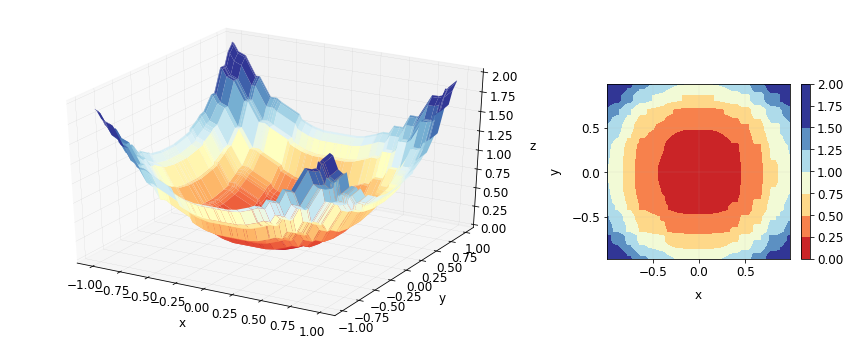
trn contains all possible pairs of 50 values for x and 50 values for y and label contains the values of \(x^2 + y^2 \) for those pairs. The data looks like this.
Boosting
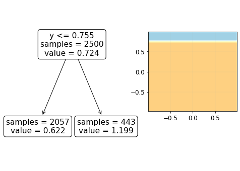
Our goal is to approximate the contour plot shown above on the right using an ensemble of weak learners. Let’s use a decision tree of depth 1 (also called a decision stump) as the weak learner. A decision stump would just divide the xy-plane into two regions based on a cutoff value for either x or y and assign one value to all the samples in one region and assign another value to all the samples in the other region. It looks something like this.
Depending upon the errors made by this decision stump, the next decision stump is made and so forth. How these errors are utilized in making the next decision stump and how the results from all the decision stumps (or in general weak learners) are combined to make one strong learner depends upon the type of boosting method used. For example, at this point, AdaBoost would give different weights to samples based on the errors made by the first decision stump, forcing itself to make the next decision stump such that it focusses more on the errors made by the first stump. The first 5 decision stumps from scikit-learn’s AdaBoostRegressor (which implements the algorithm in this paper) look like this.
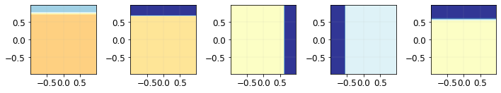
We see that each weak learner splits the xy-plane at different boundaries and assigns different values on each side of the boundary. Such weak learners are then “combined” using different weights to make one strong learner.
Gradient Boosting
Unlike AdaBoost, the most commonly used version of gradient boosting does not update the weights of the training samples based on the errors to train the next weak learner. Instead, it starts with one prediction for all the samples and additively adds weak learners (usually decision trees) that minimize the loss for a given loss function (see this for a nice overview of the math behind XGBoost, and original XGBoost manuscript if you are interested). In our example of predicting \( z\) from \(x\) and \(y\), it looks something like this

where \(f_k\) represents the decision tree (weak learner) added at step \(k\) that is constructed so as to minimize the loss between the predictions at step \(k\) (in our example, the \(\hat{z}^{(k)}\)) and the original \(z\).
In regression problems with mean squared error as the loss function of interest, this means training the next decision tree (at step \(k+1\)) to fit the residuals of predictions at step \(k\). Note that XGBoost builds decision trees in a slightly different manner than regular gradient boosting methods (that build regular decision trees) but the basic idea of gradient boosting is the same.
Let’s build a XGBoost model on the data we have using decision stumps.
import xgboost as xgb
dtrain = xgb.DMatrix(trn, label= label, feature_names=['x', 'y'])
num_round = 100
param = {'max_depth':1,
         'base_score':0, #initial prediction
         'eta':0.7, #learning rate
         'objective':'reg:squarederror',}

bst = xgb.train(param,
                dtrain,
                num_boost_round= num_round,
                evals=[(dtrain, 'train')],
                verbose_eval=20,
                early_stopping_rounds=5)
[0]	train-rmse:0.46114
Will train until train-rmse hasn't improved in 5 rounds.
[20]	train-rmse:0.08885
[40]	train-rmse:0.06455
[60]	train-rmse:0.05207
[80]	train-rmse:0.04447
[99]	train-rmse:0.03942
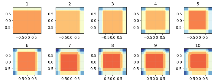
The predictions of the model using the first 10 boosted trees look like this.
We can also look at the individual trees that were trained and then used for the predictions.
fig, axs = plt.subplots(1,2)
xgb.plot_tree(bst, num_trees=0, ax=axs[0])
axs[0].set_title('k = 1')
xgb.plot_tree(bst, num_trees=1, ax=axs[1])
axs[1].set_title('k = 2')
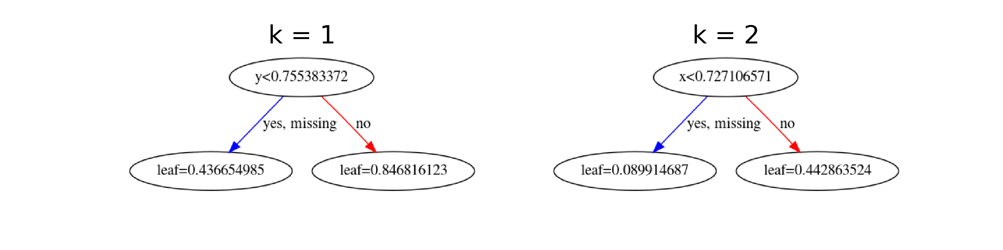
This is how the predictions look on the training data.
Now, we can use decision trees of depth more than 1 to get contour plots that look more like our original contour plot with almost concentric circles. By using trees of depth 2, we get a much better looking plot.
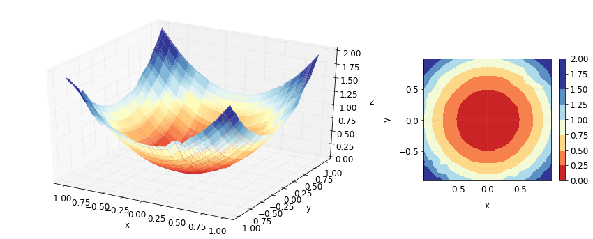
In fact, we can keep increasing the depth and our contour plots will keep getting better in this example. Here’s what we get for using trees of depth 4.

But just increasing the number of parameters to get a better fit usually leads to overfitting. Here, it was not a problem because we did not add any noise in the data - \(z\) was a deterministic function of \(x\) and \(y\). In real world problems, there is always noise. Let’s see what would happen if some noise was added and data was generated according to the equation \[ z= x^2 + y^2 + \epsilon\]
Z_noise =  X**2 + Y**2 + np.random.exponential( 0.3, (n,n))
label_noise = Z_noise.reshape(-1)
dtrain_noise = xgb.DMatrix(trn, label= label_noise, feature_names=['x', 'y'])
num_round = 10
param_reg = {'max_depth':8,
             'base_score':0,
             'eta':0.2,
             'objective':'reg:squarederror',
             'gamma':0, }

bst =  xgb.train(param_reg,
            dtrain_noise,
            num_boost_round= num_round,
            evals=[(dtrain, 'train')],
            verbose_eval=20,
            early_stopping_rounds=5)
[0]	train-rmse:0.64630
Will train until train-rmse hasn't improved in 5 rounds.
[9]	train-rmse:0.20384
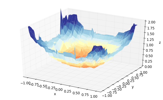
We see that in addition to capturing the real relationship between the predictors and the dependent variable, the model also starts to capture the noise in these particular samples. For this reason, we usually regularize our models. In boosting methods where tree ensembles are used, some of the most commonly used parameters for regularization are maximum tree depth, number of trees, learning rate etc. In XGBoost, we can use
eta, the learning ratemin_child_weight, which in case of regression with MSE is the number of samples required in a nodemax_depth, the maximum tree depthgamma, the minimum loss reduction required for a splitlambda, the regularization termnum_boost_round, number of treessubsample, proportion of samples used to build a treecolsample_bytree, proportion of features used to build a tree.
For instance, we can smoothen our predictions of our previous model by increasing the number of minimum samples required in a leaf node. Keeping everything else the same, the predictions from the new model look like this.
num_round = 10
param_reg = {'max_depth':8,
             'base_score':0.,
             'eta':0.2,
             'objective':'reg:squarederror',
             'min_child_weight':100}

bst =  xgb.train(param_reg,
            dtrain_noise,
            num_boost_round= num_round,
            evals=[(dtrain, 'train')],
            verbose_eval=40,
            early_stopping_rounds=5, )
[0]	train-rmse:0.64824
Will train until train-rmse hasn't improved in 5 rounds.
[9]	train-rmse:0.21758
which is a much better representation of the relationship between \(z\) and \(x,y\), even though the training loss is a bit higher than the previous model. To get a better understanding of the parameters, I recommend reading the documentation and this note. Also, there are a number of blog posts about fine-tuning hyperparameters in XGBoost which you might find helpful.
Hope this post helps you get started with boosting, gradient boosting in particular. Please note that this is by no means an exhaustive tutorial on either gradient boosting or XGBoost. Instead, treat it as a primer to dig deep into the math if you are intersted in the theoretical aspect of gradient boosting or a primer to dig deep into the features of the XGBoost library if you are more on the applied side. Please let me know if you have any suggestions or corrections for this post.