Gradient Descent Optimization in Deep Learning

As I mentioned in my previous post, gradient descent is used to optimize parameters of neural networks. There exist a number of variants of the simple gradient descent algorithm that try to optimize the training time and performance of neural networks. In my previous post, I talked about the original gradient descent using very simple examples. In this post, I will illustrate the performance of two variants - Gradient descent with momentum, and Adam - using very simple examples in two different settings.

In plain gradient descent, we calculate the gradient of the loss with respect to a parameter and subtract a proportion of the gradient from the current estimate of the parameter at each step. In gradient descent with momentum, what we subtract at each step not only depends upon the gradient at that step, but also depends upon the gradients at all previous steps. Specifically, at each step we subtract from the current estimate a weighted average of the current gradient and what was substracted in the last step. This weighted average is equivalent to a (exponentially decaying) weighted average of gradients at all the previous steps. Using momentum accelerates the progress of gradient descent by dampening the oscillations in ravines around local optima.

In momentum, all the updates are made using the same learning rate. Adaptive Moment Estimation (Adam) is a method that uses different learning rates for different parameters at different steps. In addition to keeping track of the (exponentially decaying) average of the gradients like in momentum, it also keeps track of the exponentially decaying average of the squared gradients and adapts the learning rates according to the latter. Essentially, it makes the learning rates higher for parameters with smaller average of squared gradients and smaller for parameters with high values of the average of squared gradients.

Both momentum and Adam can help converge to a local minima faster than plain gradient descent. Which is better depends upon the loss landscape i.e., the function that relates the loss to the parameters. For simple loss functions, plain gradient descent can be good enough; momentum usually accelerates the optimization of plain gradient descent, whereas Adam is generally more preferable for more complex and bumpy loss landscapes. Let’s take an example of a simple loss landscape. It looks something like this.

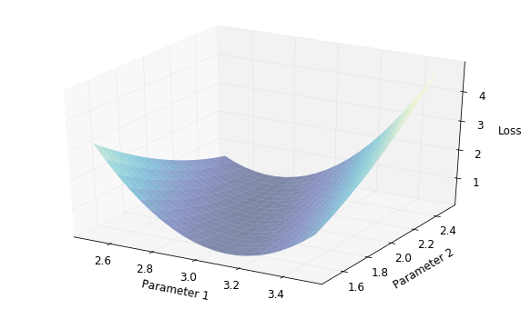
We have two parameters, one each on the x and y axes, and the loss on the z-axis. While doing gradient descent, we basically walk on surfaces like the one shown above and stop when we think we are at the lowest point. The variants of these gradient descent algorithms are different methods to decide how to walk.

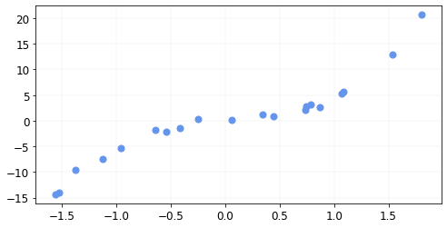
Let’s try out momentum and Adam against plain gradient descent. First, let’s consider a simple function \(y = 3x^3 + 2x + \epsilon\) and generate data for it.

n = 20
x = torch.ones(n,2) 
x[:,1].uniform_(-2.,2)
x[:,0] = x[:,1]**3
x[:5]

tensor([[ 1.2816,  1.0862],
        [ 0.0891,  0.4467],
        [-2.6153, -1.3778],
        [ 0.3921,  0.7319],
        [ 0.4149,  0.7458]])

coef = torch.tensor([3.,2]); 
errors = torch.empty(n).normal_(mean=0,std=.5)
y = x@coef + errors
y[:5]

tensor([ 5.5981,  0.9429, -9.5352,  2.0514,  2.7786])

#Make 2d tensors 
x_trn = x[:,1][:,None] 
y_trn = y[:,None]

The data looks like this

Let’s define our mean squared error

def mse(y, y_hat): return ((y - y_hat)**2).mean()

To do gradient descent, we will use pytorch. Let’s define a new model using nn.module from pytorch the parameters of which we will optimize.

class MyModel(nn.Module):
    def __init__(self, p = 3, a_start = 3., b_start = 2.): 
        super().__init__()
        self.p = p
        parms = torch.tensor([[a_start], [b_start]])
        self.coef_hat = nn.Parameter(parms)

    def forward(self, xb):
        new_x = torch.cat((xb**self.p, xb), 1) 
        return new_x@self.coef_hat 

We can set up our optimizers using plain gradient descent, momentum, and Adam using pytorch as follows:

opt  = optim.SGD(model.parameters(), lr = learn_rate ) # Gradient Descent
opt  = optim.SGD(model.parameters(), lr = learn_rate, momentum=0.9 ) # Momentum
opt  = optim.Adam(model.parameters(), lr = learn_rate ) # Adam

And we can train as usual

model = MyModel(p = 3, a_start = 2.6, b_start = 1.6)
opt = optim.SGD(model.parameters(), lr = lr, )
for i in range(25):
    y_hat = model(x_trn)
    loss = mse(y_trn, y_hat) 
    if i%5 ==0: print(f"Iteration {i}, Loss = {loss.data.item()}")
    loss.backward()
    opt.step()
    opt.zero_grad()

Iteration 0, Loss = 1.2755730152130127
Iteration 5, Loss = 1.1794413328170776
Iteration 10, Loss = 1.0930845737457275
Iteration 15, Loss = 1.0155079364776611
Iteration 20, Loss = 0.945820152759552

Let’s compare the results of the three algorithms.

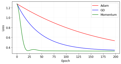
We see that using momentum, we converge much faster than plain gradient descent. On the other hand, Adam performs much worse. The loss landscape we saw in the beginning of this post was for the data generated here. Let’s see the updates at each iteration for the three algorithms.

We see that plain gradient descent slowly rolls towards the minimum (the black triangle represents the maximum likelihood estimates of \(a\) and \(b\)), whereas Momentum is fast. Momentum in fact crosses the valley because of its “momentum” and then comes back. Adam is slow in this case because the gradients are large in the beginning thus keeping the learning rates low.

Loss landscapes for most applications are not smooth and do not look like the one before. The landscapes have bumps with very high gradients. In that case, lowering the learning rate (which Adam would do in that case) can be helpful. Another situation where Adam would be helpful is when we start in a relatively small flat region of the loss landscape. Because the region is flat, the gradients would be close to zero - so plain gradient descent and momentum both will only make small updates to the estimates that will never leave that flat region. In this case, Adam would increase the learning rate (because the average of squared gradients would be small).

Let’s see this in practice. First, let’s generate some data and a function with a bumpy loss function.

Let’s create a small neural network with two hidden layers with 2 and 5 neurons respectively. Each input and output is a scalar (1d tensor). The first hidden layer does not have biases whereas the second one does.

MyBumpyModel = nn.Sequential(
                nn.Linear(1, 2,bias=False), 
                nn.ReLU6(),
                nn.Linear(2,5),
                nn.ReLU6(),
                nn.Linear(5,1),
                        )

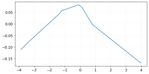
We will generate some data according to the MyBumpyModel and then pretend that we want to estimate the parameters of the first hidden layer (2 parameters) that minimize the mean squared error assuming all other parameters are fixed.

The data looks like this.

Like before, we can train our model using the three different optimizers and see the results.

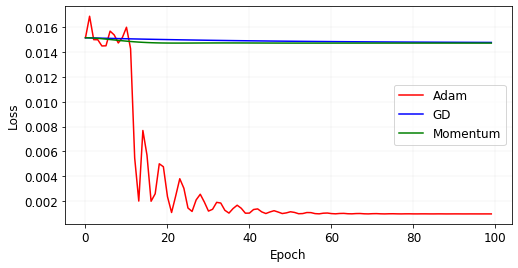
If we look at what happened here in the loss landscape, we see that our initial point was in a relatively flat area. While plain gradient descent and momentum got stuck in that flat area, Adam increased the learning rate as a result of the low average of squared gradients and was able to escape.

I hope this gives you a conceptual overview of these variants of gradient descent optimization. There are many other variants which I didn’t talk about in this post (see this post for an overview of all gradient descent optimization algorithms). Please let me know if you have any suggestions or corrections for this post.